
频率域滤波
Rotation
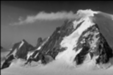
Figure. 1(b) was generated by:
1. Multiplying Fig.1 (a) by \((-1)^{x + y}\);
2. Computing the discrete Fourier transform;
3. Taking the complex conjugate of the transform;
4. Computing the inverse discrete Fourier transform;
5. Multiplying the real part of the result by \((-1)^{x + y}\).
Explain (mathematically) why Fig. 1(b) appears as it does.
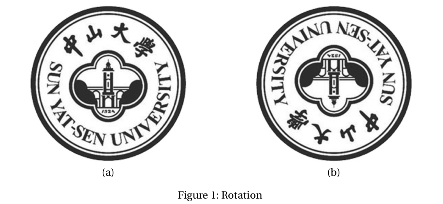
假设空间域函数为 \(f(x, y)\),频率域函数为 \(F(u, v)\)。对频率域的函数的共轭复数进行逆向傅立叶变换的过程如下:
\[\begin{align*} \widetilde{f}(x, y) &= \mathcal{F}^{-1}\{F^{*}(u, v)\}\\ &= \sum_{u = 0}^{M - 1} \sum_{v = 0}^{N - 1} F(u, v) e^{-j 2 \pi(\frac{ux}{M} + \frac{vy}{N})} \\ &= \sum_{u = 0}^{M - 1} \sum_{v = 0}^{N - 1} F(u, v) e^{j 2 \pi \left[\frac{u(-x)}{M} + \frac{v-(y)}{N} \right]} \\ &= f(-x, -y) \end{align*}\]由此可知,转换后的图像是上下、左右翻转的。
Fourier Spectrum
The Fourier spectrum in Figure. 2(b) corresponds to the original image Figure. 2(a). Figure. 2(c) is Figure. 2(a) padded with zeros, and Figure. 2(d) is the Fourier spectrum of Figure. 2(c). Explain the significant increase in signal strength along the vertical and horizontal axes of Figure. 2(d) compared with Figure. 2(b).
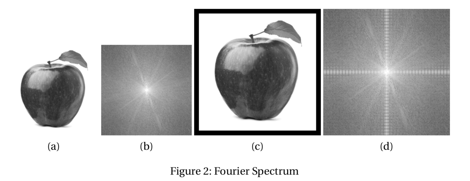
在原图像的四周填充了零值后,原图像边界部分的灰度值会产生一个较大的跳跃,这种转换导致频率域中对应的高频信号增强,最终导致傅立叶谱图像中垂直和水平方向两个轴线上的亮度增强。
Lowpass and Highpass
1). Find the equivalent Filter \(H(u,v)\) in the frequency domain for the following spatial filter:
\[\begin{bmatrix} 0 & 1 & 0 \\ 1 & -4 & 1 \\ 0 & 1 & 0 \end{bmatrix}\]由空间滤波器可知,输出的图像函数为:
\[g(x, y) = f(x - 1, y) + f(x + 1, y) + f(x, y - 1) + f(x, y + 1) - 4 f(x, y)\]对 \(g(x, y)\) 进行傅立叶变换,得到:
\[\begin{align*} G(u, v) &= \mathcal{F}\{ g(x, y) \} \\ &= \mathcal{F}\{ f(x - 1, y) \} + \mathcal{F}\{ f(x + 1, y) \} + \mathcal{F}\{ f(x, y - 1) \} + \mathcal{F}\{ f(x, y + 1) \} - 4 \mathcal{F}\{ f(x, y) \} \end{align*}\]应用傅立叶变换的平移特性 \(f(x - x_0, y - y_0) \Leftrightarrow F(u, v) e^{-j 2 \pi ( \frac{x_0 u}{M} + \frac{y_0 v}{N} )}\),得到:
\[\begin{align*} G(u, v) &= F(u, v) e^{-j 2 \pi ( \frac{u}{M})} + F(u, v) e^{j 2 \pi ( \frac{u}{M})} + F(u, v) e^{-j 2 \pi ( \frac{v}{N})} + F(u, v) e^{j 2 \pi ( \frac{v}{N})} - 4 F(u, v) \\ &= \left[ e^{-j 2 \pi ( \frac{u}{M})} + e^{j 2 \pi ( \frac{u}{M})} + e^{-j 2 \pi ( \frac{v}{N})} ++ e^{j 2 \pi ( \frac{v}{N})} - 4 \right] F(u, v) \end{align*}\]由 \(G(u, v) = H(u, v) F(u, v)\) 可得频率域滤波器:
\[H(u, v) = e^{-j 2 \pi ( \frac{u}{M})} + e^{j 2 \pi ( \frac{u}{M})} + e^{-j 2 \pi ( \frac{v}{N})} ++ e^{j 2 \pi ( \frac{v}{N})} - 4\]利用欧拉公式 \(e^{j \theta} = \cos\theta + j \sin\theta\) 可得:
\[H(u, v) = 2 \cos{\frac{2 \pi u}{M}} + 2 \cos{\frac{2 \pi v}{N}} - 4\]2). Is \(H(u,v)\) a low-pass filter or a high-pass filter? Prove it mathematically.
计算可得:\(H(0, 0) = 0\),\(H( \frac{M}{4} , \frac{N}{4} ) = -4\),\(H( \frac{M}{2} , \frac{N}{2} ) = -8\)。
当 \((u, v)\) 远离原点时,\(H(u,v)\) 的值减小,所以 \(H(u,v)\) 是低通滤波器。
Fourier Transform
Write a function to perform 2-D Discrete Fourier Transform (DFT) or Inverse Discrete Fourier Transform (IDFT). The function prototype is “dft2d(input_img, flags) → output_img”, returning the DFT / IDFT result of the given input. “flags” is a parameter to specify whether DFT or IDFT is required.
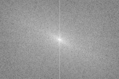
1. Perform DFT and manually paste the (centered) Fourier spectrum on your report.
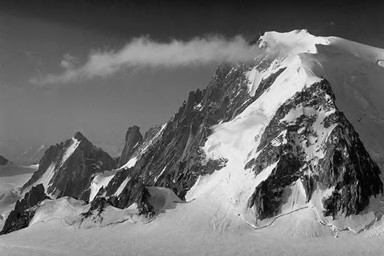
原图:

谱图:
2. Perform IDFT on the result of the last question, and paste the real part on your report. Note: the real part should be very similar to your input image.
3. Detailed discuss how you implement DFT / IDFT.
-
DFT
-
对每一行执行离散傅立叶变换。
-
对每一列执行离散傅立叶变换。
-
-
IDFT
-
对每一行执行逆向离散傅立叶变换。
-
对每一列执行逆向离散傅立叶变换。
-
def fourier_2d(matrix):
    """Compute the discrete Fourier Transform of the matrix"""
    M, N = matrix.shape
    output_matrix = np.zeros((M, N), dtype=np.complex)
    for row in range(M):
        output_matrix[row, :] = fourier_1d(matrix[row])
    for col in range(N):
        output_matrix[:, col] = fourier_1d(output_matrix[:, col])
    return output_matrix

def inverse_fourier_2d(matrix):
    """Compute the inverse discrete Fourier Transform of the matrix"""
    M, N = matrix.shape
    output_matrix = np.zeros((M, N), dtype=np.complex)
    for row in range(M):
        output_matrix[row, :] = inverse_fourier_1d(matrix[row])
    for col in range(N):
        output_matrix[:, col] = inverse_fourier_1d(output_matrix[:, col])
    return output_matrix

def fourier_1d(arr):
    """Compute the discrete Fourier Transform of the 1D array"""
    N = arr.shape[0]
    # [0, 1, 2, ... , N - 1]
    x = np.arange(N).reshape((1, N))
    # transpose of x
    u = x.reshape((N, 1))
    # e ^ (-j * 2 * π * u * x / N)
    E = np.exp(-1j * 2 * np.pi * np.dot(u, x) / N)
    return np.dot(E, arr)

def inverse_fourier_1d(arr):
    """Compute the inverse discrete Fourier Transform of the 1D array"""
    N = arr.shape[0]
    # [0, 1, 2, ... , N - 1]
    x = np.arange(N).reshape((1, N))
    # transpose of x
    u = x.reshape((N, 1))
    # e ^ (j * 2 * π * u * x / N)
    E = np.exp(1j * 2 * np.pi * np.dot(u, x) / N)
    return np.dot(E, arr) / N
Fast Fourier Transform
This is an optional task. You are required to manually implement the Fast Fourier Transform (FFT). The function prototype is “fft2d(input_img, flags)→ output_img”, returning the FFT / IFFT result of the given input. “flags” is a parameter to specify whether FFT or IFFT is required. “fft2d” should produce very similar results in comparison to “dft2d”. However, your implementation may be limited to images whose sizes are integer powers of 2. We recommend you to handle this problem by simply padding the given input so as to obtain a proper size.
For the report, please load your input image and use your program to:
1. Perform FFT and manually paste the (centered) Fourier spectrum on your report.
原图如下:
谱图如下:

2. Perform IFFT on the result of the last question, and paste the real part on your report.

3. Explain why does FFT hove a lower time complexity than DFT.
某个点 M 的傅立叶级数可以分为两个部分计算,这两个部分具有对称性,所以当求出前一个部分后,后一部分可以直接推出,而不必重复计算。通过不断地递归划分,时间复杂度会从 O(N × N) 降为 O(N × log(N))。
4. Detailed discuss how you implement FFT/IFFT.
-
FFT:
-
对每一行执行一维 FFT。
-
对每一列执行一维 FFT。
-
-
IFFT:
-
对每一行执行一维逆向 FFT。
-
对每一列执行一维逆向 FFT。
-
def fast_fourier_2d(matrix):
    """Compute the discrete Fourier Transform of the matrix"""
    M, N = matrix.shape
    output_matrix = np.zeros((M, N), dtype=np.complex)
    for row in range(M):
        output_matrix[row, :] = fast_fourier_1d(matrix[row])
    for col in range(N):
        output_matrix[:, col] = fast_fourier_1d(output_matrix[:, col])
    return output_matrix

def inverse_fast_fourier_2d(matrix):
    """Compute the inverse discrete Fourier Transform of the matrix"""
    M, N = matrix.shape
    output_matrix = np.zeros((M, N), dtype=np.complex)
    for row in range(M):
        output_matrix[row, :] = inverse_fast_fourier_1d(matrix[row])
    for col in range(N):
        output_matrix[:, col] = inverse_fast_fourier_1d(output_matrix[:, col])
    return output_matrix

def fast_fourier_1d(arr):
    """Compute the discrete Fourier Transform of the 1D array"""
    arr = np.asarray(arr, dtype=np.complex)
    N = arr.shape[0]
    if N % 2 > 0:
        return fourier_1d(arr)
    else:
        even_part = fast_fourier_1d(arr[::2])
        odd_part = fast_fourier_1d(arr[1::2])
        factor = np.exp(-1j * 2 * np.pi * np.arange(N) / N)
        return np.concatenate([even_part + factor[: N // 2] * odd_part,
                            even_part + factor[N // 2 :] * odd_part])

def inverse_fast_fourier_1d(arr):
    """Compute the inverse discrete Fourier Transform of the 1D array"""
    def rec(arr):
        arr = np.asarray(arr, dtype=np.complex)
        N = arr.shape[0]
        if N % 2 > 0:
            return inverse_fourier_1d(arr) * N
        else:
            even_part = rec(arr[::2])
            odd_part = rec(arr[1::2])
            factor = np.exp(1j * 2 * np.pi * np.arange(N) / N)
            return np.concatenate([even_part + factor[: N // 2] * odd_part,
                                even_part + factor[N // 2 :] * odd_part])
    return rec(arr) / arr.shape[0]
Filtering in the Frequency Domain
Write a function that performs filtering in the frequency domain. The function prototype is “filter2d_freq(input_img, filter) → output_img”, where “filter” is the given filter. You can modify the prototype if necessary. According to the convolution theorem, filtering in the frequency domain requires you to apply DFT / FFT to the given image and filter, and then multiply them, followed by IDFT / IFFT to get the filtered result. Hence, it should be easy to implement “filter2d_freq” based on “dft2d” (or “fft2d”).
For the report, please load your input image and use your “filter2d_freq” function to:
1. Smooth your input image with an 5 × 5 averaging filter. Paste your result on the report.
2. Sharpen your input image with the following 3 × 3 Laplacian filter and then paste the result.
3. Detailed discuss how you implement the filtering operation function in less than 2 pages.
-
填充图像,将图像移至变换的中心,并对图像做 DFT。
-
填充滤波器,将滤波器移至变换的中心,并对滤波器做 DFT。
-
将图像与滤波器相乘。
-
对上一步的乘积求 IDFT。
-
取上一步结果的实部,并通过变换将结果移至矩阵的左上角。
-
取出上一步结果的左上角,恢复图像为原来的大小。
def filter2d_freq(matrix, filter):
    M, N = matrix.shape
    M_f, N_f = filter.shape
    P, Q = M * 2, N * 2

    # padded matrix
    pad_matrix = np.zeros((P, Q))
    pad_matrix[:M, :N] = matrix
    # shifted matrix
    shifted_matrix = shift(pad_matrix)
    # fft matrix
    fft_matrix = dft2d(shifted_matrix, 'FFT')

    # padded filter
    pad_filter = np.zeros((P, Q))
    pad_filter[:M_f, :N_f] = filter
    # shifted filter
    shifted_filter = shift(pad_filter)
    # fft filter
    fft_filter = dft2d(shifted_filter, 'FFT')

    # filtering in the Frequency Domain
    g_matrix = fft_matrix * fft_filter

    # ifft
    ifft_matrix = dft2d(g_matrix, 'IFFT')
    # shift ifft matrix
    shifted_ifft_matrix = shift(ifft_matrix)
    return shifted_ifft_matrix.real[:M, :N]

def shift(matrix):
    M, N = matrix.shape
    x = np.arange(M).reshape((M, 1))
    y = np.arange(N).reshape((1, N))
    return (-1) ** (x + y) * matrix